Biology is notorious for its exuberant abundance of factors, and one of its central challenges is to discover which among a large group of factors are important for a given question. For this reason, biologists spend a lot of time looking at tables that might resemble this one :

Which factors are important? Which differences among samples are important? There are a variety of mathematical tools that can help distill these tables into something perhaps more tractable to interpretation. One way or another, all of these tools work by decomposing the data into vectors and projecting them into a lower dimensional space, much the way object casts a shadow onto a surface. 

http://www.flickr.com/photos/violentz/1908351694/

The idea is to find a projection that highlights an important feature of the original data. For example, the projection of the fire hydrant onto the pavement highlights its bilateral symmetry.

So, projections are very useful. Many people have a favorite projection, and like to apply the same one to every bunch of data they encounter. This is better than just staring at the raw data, but different data and different effects lend themselves to different projections. It would be better if people generalized their thinking a little bit.

When you make a projection, you really have three choices. First, you have to choose how the data fits into the original space. There is more than one valid way of thinking about this. You could think about it as arranging the elements into vectors, or deciding what “reshuffling” operations are allowed. Then, you have to choose what kind of projection you want to make. Usually people stick with some flavor of linear transformation. Last, you have to choose the space you want to make your projection into. What dimensions should it have? What relationship should it have with the original space? How should it be oriented?

In the photograph of the fire hydrant, the original data (the fire hydrant) is embedded in a three dimensional space, and projected onto the ground (the lower dimensional space) by the sunlight by casting a shadow. The ground happens to be roughly orthogonal to the fire hydrant, and the sunlight happens to fall from a certain angle. But perhaps this is not the ideal projection. Maybe we’d get a more informative projection if we put a vertical screen behind the fire hydrant, and used a floodlight? Then we’d be doing the same transformation on the same representation of the data, but into a space with a different orientation. Suppose we could make the fire hydrant semi-transparent, we placed it inside a tube-shaped screen, and illuminated the fire hydrant from within? Then we’d be using a different representation of the original data, and we’d be doing a non-linear projection into an entirely different space with a different relationship with the original space. Cool, huh?

It’s important to think generally when choosing a projection. When you start trying to tease some meaning out of a big data set, the choice of principal component analysis, or k-means clustering, or canonical correlation analysis, or support vector machines, has important implications for what you will (or won’t) be able to see.

How we started this collaboration: a DARPA project named FunBio

Between 2005 and 2011, DARPA had a program humbly named The Fundamental Laws of Biology (FunBio). The idea was to foster collaborations among mathematicians, experimental biologists, physicists, and theoretical biologists — many of whom already bridged the gap between modeling and experiment. Simon Levin was the PI of the project and Benjamin Mann was the program officer. The group was large enough to have a number of subgroups that included theorists and empiricists, including a group focused on ecology. Jonathan Eisen was the empiricist for microbial ecology, and was very interested in the binning problem for metagenomics; that is, classifying reads, usually by taxonomy. Conversations in and out of the program facilitated the parallel development of two methods in this area: LikelyBin (led by Andrey Kislyuk and Joshua Weitz with contributions from Srijak Bhatnagar and Jonathan Dushoff) and CompostBin (led by Sourav Chatterji and Jonathan Eisen with contributions from collaborators). At this stage, the focus was more on methods than biological discoveries.

The binning problem highlights some fascinating computational and biological questions, but as the program developed, the group began to tilt in direction of biological problems. For example, Simon Levin was interested in the question: Could we identify certain parts of the ocean that are enriched for markers of social behavior?

One of the key figures in any field guide is a ecosystem map. These maps are the starting point from which a researcher can orient themselves when studying an ecosystem by placing their observations in context. 

There are a variety of approaches one could take that entail deep questions about how best to describe variation in taxonomy and function. For example, we could try to find “canonical” examples of each ecosystem, and then perhaps identify intermediates between them. Similarly, we could try and find “canonical” examples of the way different functions are distributed across ecosystem and identify intermediates between them.

In the discussions that followed, we discussed how to describe the functional and taxonomic diversity in a community as revealed via metagenomics; that is, how do we describe, identify and categorize ecosystems and associated function? In order to answer this question, we had to confront a difficult issue: how to quantify and analyze metagenomic profile data.

Metagenomic profile data: making sense of complexity at the microbe scale

Metagenomics is perhaps the most pervasive cause of the proliferation of giant tables of data that now beset biology. These tables may represent the proportion of taxa at different sites, e.g., as measured across a transect using effective taxonomic units as proxies for distinct taxa. Among these giant tables, one of the challenges that has been brought to light is that there can be a great deal of gene content variability among individuals of an individual taxa. As a consequence, obtaining the taxonomic identities of organisms in an ecosystem is not sufficient to characterize the biological functions present in that community. Furthermore, ecologists have long known that there are often many organisms that could potentially occupy a particular ecological niche. Thus, using taxonomy as a proxy for function can lead to trouble in two different ways; the organism you’ve found might be doing something very different from what it usually does, and second, the absence of an organism that usually performs a particular function does not necessarily imply the absence of that function. So, it’s rather important to look directly at the genes in the ecosystem, rather than taking proxies. You can see where this is going, I’m sure: Metagenomics, the cure for the problems raised by metagenomics!

When investigating these ecological problems, it is easy to take for granted the ability to distinguish one type of environment from another. After all, if you were to wander from a desert to a jungle, or from forest to tundra, you can tell just by looking around what kind of ecosystem you are in (at least approximately). Or, if the ecosystems themselves are new to you, it should at least be possible to notice when one has stepped from one into another. However, there is a strong anthropic bias operating here, because not all ecosystems are visible on humans scales. So, how do you distinguish one ecosystem from another if you can’t see either?

One way is to look at the taxa present, but that works best if you are already somewhat familiar with that ecosystem. Another way is to look at the general properties of the ecosystem. With microbial ecosystems, we can look at predicted gene functions. Once again, this line of reasoning points to metagenomics.

We wanted to use a projection method that avoids drawing hard boundaries, reasoning that hard boundaries can lead to misleading results due to over-specification. Moreover, in doing so Jonathan Dushoff advocated for a method that had the benefits of “positivity”, i.e., the projection would be done in a space where the components and their weights were positive, consistent with the data, and which would help the interpretability of our results. This is the central reason why we wanted to use an alternative to PCA. The method Jonathan Dushoff suggested was Non-negative Matrix Factorization (NMF). This choice led to a number of debates and discussions, in part, because NMF is not a “standard” method (yet). Though, it has seen increasing use within computational biology: http://www.ploscompbiol.org/article/info%3Adoi%2F10.1371%2Fjournal.pcbi.1000029. It is worth talking about these issues to help contextualize the results we did find.

The Non-negative Matrix Factorization (NMF) approach to projection

The conceptual idea underlying NMF (and a few other dimensional reduction methods) is a projection that allows entities to exist in multiple categories. This turns out to be quite important for handling corner cases. If you’ve ever tried to build a library, you’ve probably encountered this problem. For example, you’ve probably created categories like Jazz, Blues, Rock, Classical and Hip Hop. Inevitably, you find artists who don’t fit into the scheme. Does Porgy and Bess go into Jazz or Opera? Does the soundtrack for Rent go under Musicals or Rock? What the heck is Phantom of the Opera anyway? If your music library is organized around a hierarchy of folders, this can be a real headache, and either results either in sacrificing information by arbitrarily choosing one legitimate classification over another, or in creating artistically meaningless hybrid categories.

This problem can be avoided by relaxing the requirement that each item must belong to exactly one category. For music libraries, this is usually accomplished by representing categories as attribute tags, and allowing items to have more than one tag. Thus, Porgy and Bess can carry the tags Opera, Jazz and Soundtrack. This is more informative and less brittle.

NMF accomplishes this by decomposing large matrices into smaller matrices with non-negative components. These decompositions often do a better job at clustering data than eigenvector based methods for the same reason that tags often work better for organizing music than folders. In ecology, the metabolic profile of a site could be represented as a linear combination of site profiles, and the site profile of a taxonomic group could be represented as a linear combination of taxonomic profiles. When we’ve tried this, we have found that although many sites, taxa and Pfams have profiles close to these “canonical” profiles, many are obviously intermediate combinations. That is to say, they have characteristics that belong to more than one classification, just as Porgy and Bess can be placed in both Jazz and Opera categories with high confidence. Because the loading coefficients within NMF are non-negative (and often sparse), they are easy to interpret as representing the relative contributions of profiles.

What makes NMF really different from other dimensional reduction methods is that these category “tags” are positive assignments only. Eigenvector methods tend to give both positive and negative assignments to categories. This would be like annotating Anarchy in the U.K. by the Sex Pistols with the “Classical” tag and a score of negative one, because Anarchy in the U.K. does not sound very much like Frédéric Chopin’s Tristesse or Franz Liszt’s Piano Sonata in B minor. While this could be a perfectly reasonable classification, it is conceptually very difficult to wrap one’s mind around concepts like non-Punk, anti-Jazz or un-Hip-Hop. From an epistemological point of view, it is preferable to define things by what they are, rather than by what they are not.

To give you an idea of what this looks like when applied to ecological data, it is illustrative to see how the Pfams we found in the Global Ocean Survey cluster with one another using NMF, PCA and direct similarity:

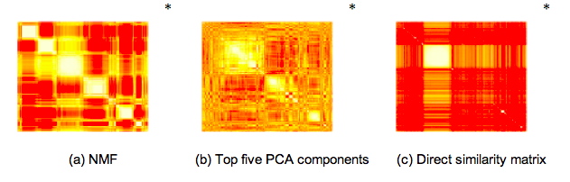
While PCA seems to over-constrain the problem and direct similarity seems to under-constrain the problem, NMF clustering results in five or six clearly identifiable clusters. We also found that within each of these clusters one type of annotated function tended to dominate, allowing us to infer broad categories for each cluster: Signalling, Photosystem, Phage, and two clusters of proteins with distinct but unknown functions. Finally – in practice, PCA is often combined with k-means clustering as a means to classify each site and function into a single category. Likewise, NMF can be used with downstream filters to interpret the projection in a “hard” or “exclusive” manner. We wanted to avoid these types of approaches.

Indeed, some of us had already had some success using NMF to find a lower-dimensional representation of these high-dimensional matrices. In 2011, Xingpeng Jiang, Joshua Weitz and Jonathan Dushoff published a paper in JMB describing a NMF-based framework for analyzing metagenomic read matrices. In particular, they introduced a method for choosing the factorization degree in the presence of overlap, and applied spectral-reordering techniques to NMF-based similarity matrices to aid in visualization. They also showed a way to robustly identify the appropriate factorization degree that can disentangle overlapping contributions in metagenomics data sets.

While we note the advantages of NMF, we should note it comes with caveats. For example, the projection is non-unique and the dimensionality of the projection must be chosen carefully. To find out how we addressed these issues, read on!

Using NMF as a tool to project and understand metagenomic functional profile data

We analyzed the relative abundance of microbial functions as observed in metagenomic data taken from the Global Ocean Survey dataset. The choice of GOS was motivated by our interest in ocean ecosystems and by the relative richness of metadata and information on the GOS sites that could be leveraged in the course of our analysis. In order to analyze microbial function, we restricted ourself to the analysis of reads that could be mapped to Pfams. Hence, the matrices have columns which denote sampling sites, and rows which denote distinct Pfams. The values in the cell denotes the relative number of Pfams matches at that site, where we normalize so that the sum of values in a column equals 1. In total, we ended up mapping more than six million reads into a 8214 x 45 matrix.

We then utilized NMF tools for analyzing metagenomic profile matrices, and developed new methods (such as a novel approach to determining the optimal rank), in order to decompose our very large 8214 x 45 profile matrix into a set of 5 components. This projection is the key to our analysis, in that it highlights the most of the meaningful variation and provides a means to quantify that variation. We spent a lot of time talking among ourselves, and then later with our editors and reviewers, about the best way to explain how this method works. Here is our best effort from the Results section that explains what these components represent :

Each component is associated with a “functional profile” describing the average relative abundance of each Pfam in the component, and with a “site profile”, describing how strongly the component is represented at each site. 

A component has both a column vector representing how much each Pfam contributes to the component and a row vector representing the importance of that component at different sites. Each Pfam may be associated with more than one component. Likewise, each component can have a different strength at each site. Remember, the music library analogy? This is how NMF achieves the effect of category “tags” which can label overlapping sets of items, rather than “folders” which must contain mutually exclusive sets.

Such a projection does not exclusively cluster sites and functions together. We discovered five functional types, but we are not claiming that any of these five functional types are exclusive to any particular set of sites. This is a key distinction from concepts like enterotypes.

What we did find is that of these five components, three of them had an enrichment for Pfams whose ontology was often identified with signalling, phage, and photosystem function, respectively. Moreover, these components tended to be found in different locations, but not exclusively so. Hence, our results suggest that sampling locations had a suite of functions that often co-occurred there together.

We also found that many Pfams with unknown functions (DUFs, in Pfam parlance) clustered strongly with well-annotated Pfams. These are tantalizing clues that could perhaps lead to discovery of the function of large numbers currently unknown proteins. Furthermore, it occurred to us that a larger data set with richer metadata might perhaps indicate the function of proteins belonging to clusters dominated by DUFs. Unfortunately, we did not have time to fully pursue this line of investigation, and so, with a wistful sigh, we kept in the the basic idea, with more opportunities to consider this in the future. We also did a number of other analyses, including analyzing the variation in function with respect to potential drivers, such as geographic distance and environmental “distance”. This is all described in the PLoS ONE paper.

So, without re-keying the whole paper, we hope this story-behind-the-story gives a broader view of our intentions and background in developing this project. The reality is that we still don’t know the mechanisms by which components might emerge, and we would still like to know where this this component-view for ecosystem function will lead. Nevertheless, we hope that alternatives to exclusive clustering will be useful in future efforts to understand complex microbial communities.

---

Full Citation: Jiang X, Langille MGI, Neches RY, Elliot M, Levin SA, et al. (2012) Functional Biogeography of Ocean Microbes Revealed through Non-Negative Matrix Factorization. PLoS ONE 7(9): e43866. doi:10.1371/journal.pone.0043866.

---